8. Output Views and Printing

cocoaNEC takes the information from your spreadsheet and translates that into a NEC-2 input "deck." cocoaNEC then sends the deck to the NEC-2 engine for execution, and finally post-processes the output from NEC-2 so the data can be viewed graphically in the Output Window.

You have already seen the SWR and elevation views in the previous three chapters.

The post-processor makes separate copies of data for each antenna model. (If you need to save two separate runs from the same model, you can make a duplicate of the model first and make changes to it. The post-processor will treat the duplicate antenna as a different model.)

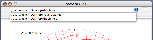
You can switch the output window to inspect the output of each antenna by selecting the model from the menu at the top of the window.



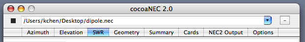
You can use the minus button to the right of the menu to remove the currently selected model from the output window.


Adding a Reference

You can designate any model in the output list to be the "reference" antenna. When you do that, the reference's radiation pattern will be superimposed on the radiation pattern of the currently selected antenna.

If you have followed the tutorial up to this point, there should be two models in the post-processor -- a dipole and a simple Yagi-Uda.

Let us now designate the dipole model as the reference.

(If you no longer have the dipole model in the output menu, don't worry. Simply Open the dipole model again, hit the Run button from the dipole's window and both the dipole and the Yagi models should now be available in the menu.)

Select the dipole model to be the one that is displayed in the output window, its data should show up the the output window.

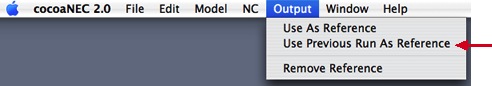
Now go to the Output Menu in the Menu Bar and choose Use As Reference.



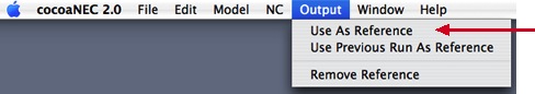
A small black square should appear to the left of the menu indicating that the dipole model has been selected as the reference, as shown below:




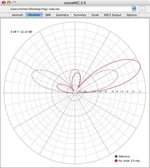
Next, switch the menu of the Output window to again look at the Yagi model. You should now see this:



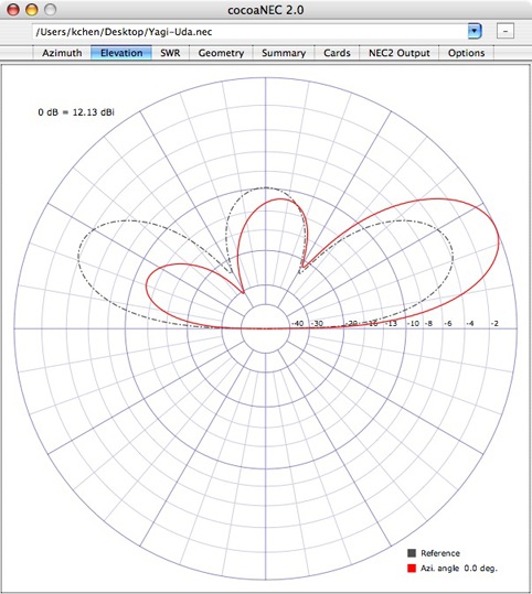
In addition to the pattern for the Yagi, you will also see the pattern for the reference antenna plotted in a dark gray dashed line.

If you wish to remove the reference antenna, select Remove Reference in the Model Menu.

Instead of superimposing a different antenna model as the reference, you can also superimpose a previous run of the same model.



Each time you run the same model, the previous run will show up as a "reference" plot. This allows you to better judge if the model is improving.


Changing the Plot Scale

There are a couple of options you can choose to control how the post-processed data is displayed. These options are available in the Options view of the output window which you can view using the rightmost tab in the row of buttons.



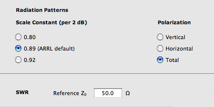
Notice in the elevation pattern above that the diameter of the -10 dB circle in the antenna pattern is half of the diameter of the outer 0 dB circle. This is the usual logarithmic scale factor (0.89 per 2 dB) that is used in most ARRL publications. It gives a moderately balanced view of both the the response near 0 dB and the back of lobes.

If you are more interested in inspecting what happens near 0 dB, change the scale constant in the Options view to 0.80 per 2 dB.

The Elevation plot changes to this:



The region between 0 and -10 dB is now stretched out in the plot. Similarly, if you wish to stretch the region that is past -10 dB, simply change the pattern scale constant to 0.92.

Notice that you can also select which polarization of the radiation field to plot from the selections in the Options tab view.


Geometry and Currents

You can inspect the geometry and currents in the wires in the Geometry view.



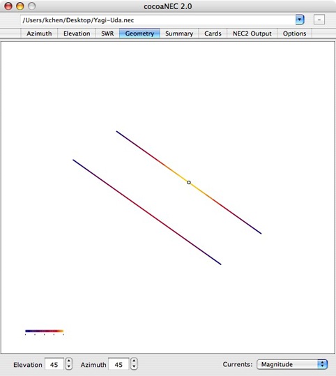
The two fields at the bottom left of the window controls the viewing angle relative to the centroid of the antenna. An elevation angle of 0 places the eye at the same height as the centroid. An elevation angle of 90 degrees corresponds to placing the eye straight above the centroid and looking back at the antenna from the +z axis. An elevation angle of -90 degrees corresponds to placing the eye below the centroid and looking up at the antenna from the -z axis.

An azimuth angle of 0 corresponds to placing the eye on the +x axis and looking back at the antenna. An azimuth angle of 90 degrees corresponds to placing the eye on the +y axis.

You can either set the angle by typing directly into the fields, or by using the up and down stepper arrow buttons. The buttons autorepeat, so you can hold down the button and see an animation. The elevation angle has hard stops at -90 degrees and +90 degrees. The azimuth angle wraps around the circle, with 360 degrees wrapping back to 0.

The Currents menu at the bottom right of the window can be set to None, Magnitude, Magnitude and Phase, and Magnitude and Relative Phase.

With the Currents menu set to None, antenna current information is not plotted. When the Currents menu is set to Magnitude, the colors of the antenna segments correspond to the magnitudes of the current. Maximum current appears as a bright yellow and zero current appears as dark gray. A scale is shown on the bottom left corner of the view.

When the menu is set to Magnitude and Phase, the currents appear as colors in the HSV color space. The phase angle of a current corresponds to the hue of the color, and the magnitude of a current corresponds to the value of the HSV color (brighter colors carry larger currents). The colors that correspond to the various phase angles for the maximum current are shown in the color wheel on the bottom left corner of the view.

The following shows the Magnitude and Phase view of a Half Square antenna with a reflector:



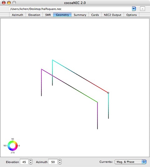
The Magnitude and Relative Phase setting is similar to the Magnitude and Phase setting except all phase angles are referenced to the phase of the current in the segment with the largest current.



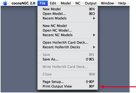
Printing an Output View

You can print the view that is currently displaying in the Output window by selecting Print Output View in the File Menu. The standard Mac OS X printer dialog will appear and you can choose to print, to preview or to generate a PDF file to be saved (or sent as FAX or email). The output can also be scaled or rotated in Page Setup... of the File Menu.

Next: Grounds and Radials...