6. Modifying the Model


If we prefer a resonant antenna, we can now modify the model by lengthen the dipole element.

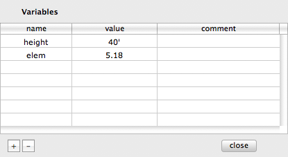
Recall that length of the dipole is determined the "y1" and "y2" values in the spreadsheet, and the formulas for them came from the positive and negative values of the variable "elem."

Open the Variables sheet again (using the Variables button in the spreadsheet window) and change the value of the variable "elem" from 5 to 5.18 (meters).



You can now close the Variables sheet and hit the Run button. Instead of doing that however, here is a shortcut.

Note that because Mac OS X sheets are modal by nature, you have to first close the Variables sheet before the you can click on the Run button in the spreadsheet.

Having to close the Variables sheet before being able to use the Run button can be cumbersome when you are trying to make quick changes to a variable while matching some criteria in the output. If you don't need to change the formula in the spreadsheet and only need need to change a variable, just keep the Variables sheet open and select Run Model from the Model Menu. You can also use the Command-R keyboard shortcut to execute a "run" more rapidly.

Hit Command-R now. You should see the SWR plot change to the following figure (yes, that is all there is to it!).



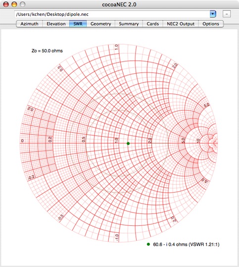
The reactance of the feed point is now down to 0.4 ohms (capacitive) and the dipole is practically resonant.

You can look at other output from the model by selecting the different tab buttons in the Output window. If you select the Elevation tab view, you will see a far field elevation plot:



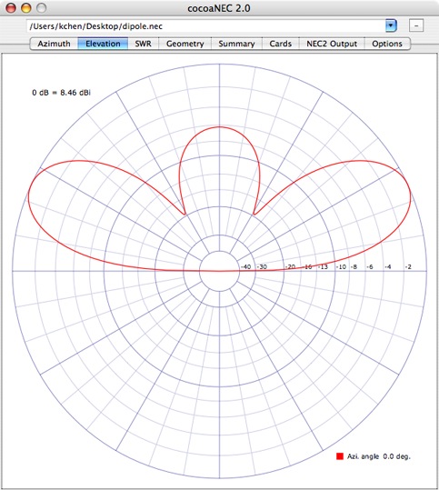
For the figure above, NEC-2 had generated the elevation plot for an azimuth angle of 0 degrees (the direction of the x axis of the antenna). The caption at the top left corner tells you that the maximum gain (the outer "0 dB" circle) for this azimuth angle is 8.46 dB over a theoretical isotropic antenna. The plot shows that the peak gain occurs at the elevation angle of about 25 degrees above the horizon.

You can tell NEC-2 to generate radiation patterns for other azimuth and elevation angles by changing the selection in the Output Control sheet in the spreadsheet.

The Output Control sheet is brought up by clicking on the Output Control button in the spreadsheet window. It is to the right of the Variables button. After changing the azimuth and elevation parameters, close the Output Control sheet and click on the Run button again. cocoaNEC will ask NEC-2 to generate a new set of output with the new parameters that you've just specified. There are some default angles in the azimuth and elevation output control; you can replace them with any angle that you wish.

So far, we have been using the default frequency (14.080 MHz) as the analysis frequency. You can choose any other frequency that you wish by opening the Environment sheet, selecting the first (Frequency) radio button and entering the frequency in the text field. Remember to use units of MHz.



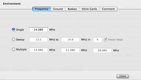
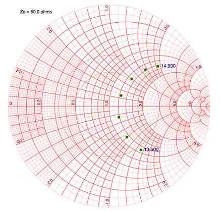
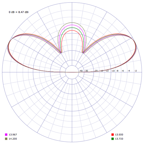
You can also ask cocoaNEC to generate a sweep between two frequency limits. If you select the Sweep radio button and set the lower frequency to 13.5 MHz and the upper frequency to 14.9 MHz, with 7 linear steps, the follow will result when you run the model of the 20m dipole.



Multiple radiation patterns are also generated (but limited to 4 frequency steps):



Notice that we could also select Multiple for the frequency selection in the environment sheet. With that, we can enter up to three unrelated frequencies. This feature could be useful when you are designing a multi-band antenna. If you need only two unrelated frequencies, just leave one of the three fields blank.

Before we proceed in our tutorial, set the frequency setting back to the single 14.080 MHz frequency.

You can superimpose up to three patterns in the azimuth and elevation plots by selecting more than one azimuth or elevation angle in the Output Control sheet. In the next chapter of the tutorial, you will see how you can also superimpose the pattern from a different antenna that you designate as a reference.

Thus far, you have created a dipole model from scratch, given it a feed point, looked at the output from NEC-2 and modified the length of the dipole so that it became resonant. We will next see how you can build upon this basic dipole.

But first, go to the File Menu and do a Save...

Next: Extending a Model...