3. Setting Feedpoints and Frequencies in NC
Notice that when you wrote the statement
voltageFeed( driven, 1.0, 0.0 ) ;
that you are simply attaching a voltage source to the center of a wire element variable that is called driven. This wire element is assigned to the wire() function by the statement
driven = wire( 0, -length, height, ...
The variable driven is itself declared as a wire element in the declaration
element driven ;
As we will see later, you can also attach a current source instead of a voltage source to the center of a wire element.
What do you do if you want to offset feed a wire instead of feeding it at the center? You simply construct the wire in two pieces that share a common endpoint. Wires that are close enough will be connected by NEC-2. This is what the NEC-2 manual has to say about how wires connect:
... segments that are electrically connected
must have coincident end points. If segments intersect other than at their
ends, the NEC code will not allow current to flow from one segment to the
other. Segments will be treated as connected if the separation of their ends
is less than about 0.001 times the length of the shortest segment.
For example, if you wish to feed an 8 meter long wire at a point 25% from one end, you can model the wire as,
element fedWire ;
fedWire = wire( 0, 0, height, 0, 4.0, height, #14, 21 ) ;
wire( 0, 4.0, height, 0, 8.0, height, #14, 21 ) ;
voltageFeed( fedWire, 1.0, 0.0 ) ;
Notice from the above example that you do not need to assign a name to every wire. You need to only do it if you want to add other properties, such as a voltage feed, to that wire. You can always assign a name to a wire and not reference it again, as a documenting tag.
You can also use a double slash to add your own comments (with no space character between the two slash characters). All characters from the double slash until the end of a line are ignored by NC. For example, the above could be written as:
element fedWire ;
// 8 metre wire made up of two 4m pieces
fedWire = wire( 0, 0, height, 0, 4.0, height, #14, 21 ) ;
wire( 0, 4.0, height, 0, 8.0, height, #14, 21 ) ; // this piece is not fed
voltageFeed( fedWire, 1.0, 0.0 ) ;
Setting Frequencies
Notice in the dipole example in the previous page that the program makes no mention of the frequency the antenna analysis is made at.
If you were to go to the Summary tab of the Output Window, you will see that NC has defaulted to using 14.080 MHz.
To use any other frequency, simply use the setFrequency function call from anywhere inside the model block. The argument of the setFrequency function is expressed in MHz. For example, the following will perform analysis at 14.100 MHz instead.
model ( "dipole" )
{
real height, length ;
element driven ;
height = 40' ;
length = 5.0 ;
driven = wire( 0, -length, height, 0, length, height, #14, 21 ) ;
voltageFeed( driven, 1.0, 0.0 ) ;
setFrequency( 14.1 ) ;
}
In fact, you can ask NC to provide multiple analysis in a single output plot by the addition of addFrequency function calls. As an example, the following will run four frequency passes in NEC-2:
model ( "dipole" )
{
real height, length ;
element driven ;
height = 40' ;
length = 5.0 ;
driven = wire( 0, -length, height, 0, length, height, #14, 21 ) ;
voltageFeed( driven, 1.0, 0.0 ) ;
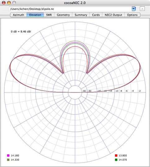
setFrequency( 13.8 ) ;
addFrequency( 14.070 ) ;
addFrequency( 14.180 ) ;
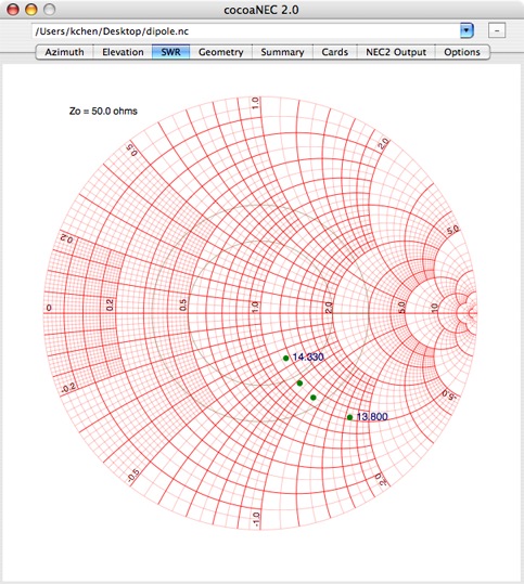
addFrequency( 14.330 ) ;
}
When you click Run on the NC window, the Elevation plot of the Output window should show the following:
The SWR view in the output window should also show the trajectory of the above frequencies:
The argument to the setFrequency or addFrequency functions need not be a constant, it can be a real varaible.
Radiation Patterns
You will probably notice by now that the radiation patterns that are generated by our simple program are plotted for fixed directions. NC defaults to generating a radiation pattern for an azimuth angle of 0 degrees (the direction of the +x axis) and it defaults to generating a radiation pattern for an elevation of 20 degrees above the horizon.
To change from the defaults, you can use the azimuthPlotForElevationAngle and the elevationPlotForAzimuthAngle function calls. Both functions take as arguments their respective angles in degrees. Elevation angles are measured from the horizon upwards and azimuth angles start with the x axis (the y axis corresponds to 90 degrees azimuth).
model ( "dipole" )
{
real height, length ;
element driven ;
height = 40' ;
length = 5.0 ;
driven = wire( 0, -length, height, 0, length, height, #14, 21 ) ;
voltageFeed( driven, 1.0, 0.0 ) ;
setFrequency( 14.040 ) ;
azimuthPlotForElevationAngle( 22.5 ) ;
elevationPlotForAzimuthAngle( 15.0 ) ;
}
As with the setFrequency function call, you can issue multiple ...PlotFor... function calls to get multiple plots that are superimposed on a single view.
A caveat is that, to reduce confusion in the Output Window, you cannot issue multiple setFrequency and multiple ...PlotFor... calls simultaneously.