When you click the Run button (command-G) in the NC window, the NC compiler will parse your program and create dictionaries to hold your variables, and a data structure in the form of a directed acyclical graph (DAG) to hold the statements and expressions of your program.
If a syntax error (or any error such as missing variable declarations, etc) is detected, NC will not proceed to the execution phase. Instead, NC will automatically bring up the Listing panel and try to display the error, as explained at the end of this page.
If NC succeeds with parsing the model into a DAG, it will then execute the code presented by the DAG from the top of the graph, i.e., where your program starts with the 'model' function header.
Even when NC successfully executes your program, it does not necessarily mean that the antenna description will generate a good card deck, that when passed to the NEC-2 engine, will send output to the Output window.
Some common errors are for example a failure to include a voltage or current feed statement, placing a wire too close to ground, etc. If the NEC-2 engine fails during execution, cocoaNEC will warn you that a failure has occurred. If you are missing a feed point, the NEC-2 engine will still succeed but the radiation patterns and SWR plot will be empty -- in those cases, you can inspect the card deck and NEC-2 output in the Output window to attempt to figure out what is wrong.
NC accumulates data for creating the "cards" for the NEC-2 card deck as it executes the statements in your program. The actual cards are not produced until NC reaches the end of the model, since comment, geometry and control cards in the NEC-2 deck have to be separated into their individual sections of the deck.
Each wire function call will create one "geometry" card. Each voltageFeed function call will create a "control" card. The geometry and excitation cards will appear at different parts of the deck even if the two system calls are next to one another. A currentFeed call will cause NC to create both geometry cards and excitation cards. Again, the cards will be separated in the deck even if they are created by a single currentFeed call.
NC will create some default output (ground parameters, frequency of the source, antenna patterns) even if your program does not explicitly create them.
When NC finishes execution and a card deck is created, cocoaNEC will pass this deck as input to the NEC-2 engine. NC's job is completed at this point, and it is left to the rest of the cocoaNEC application to present NEC-2 output in the Output window.
Optimizing Loops
If your program also includes a control function in addition to a model function, NC will start the execution at the top of the control function instead of at the top of the model function.
Take the following example:
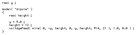
Since there is no control function in the above example, NC will simply start execution at the top of the model function. The first item in the DAG will be the one that is created by the "y=5.0" statement.
If you now add a control function, as in the example below, NC will instead start execution at the top of the control function.
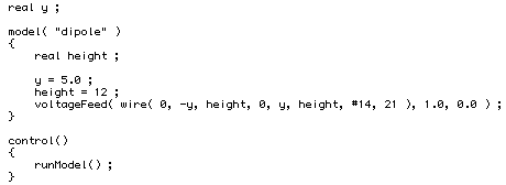
Notice in the above example that the control function contains a single function, in the form of a runModel system call. When NC encounters a runModel call, it will transfer execution to the top of the model function. When NC finishes with model, it will return to the control function.
In this above example, your program will do precisely what the previous program (that does not have a control function) will do, i.e., execute the model once.
If the control function contains a second runModel, NC will again transfer execution to the model.
Remember that once NC reaches the end of the model function, it will create a card deck and then start the NEC-2 engine which in turn will produce output in the Output window. Because of this, a new output will be generated for each runModel that is encountered.
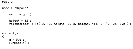
Calling runModel twice is not very useful unless you can also change some parameter in the model. The way for the control function to change a parameter in the model is to use a shared global variable. We already had a global variable called y. Notice that instead of setting the value of y inside the model itself, we can set the value of y in the control function, like so:
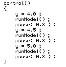
Now, take a look at the next example:
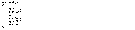
Notice that we called runModel three times from the control function, the first time after setting the value of y to 4.0, the next time after setting the value of y to 4.5 and finally after setting the value of y to 5.0. If you run this code, and if your machine is not too fast, you can actually see the VSWR move at the end of each runModel call.
In fact, NC has a special function called pause that you can use to inject a pause (in seconds or fractions of a second) to slow down the animation on the Output window.
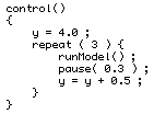
Using NC's repeat loops, the above could be simplified to:
Functions and Variables to Access NEC-2 Output
In the above examples, we are simply running loops regardless of the outcome. It is useful to watch the trajectories of VSWR animated as a movie, but it does not help with automatic optimization of antennas. To do that we will need to be able to access some numbers from the NEC-2 result.
NC has some special variables and functions which allow you to access some of NEC-2's output (this list might expand in the future).
Please note that these functions and variables can only be accessed from the control function; they cannot be accessed from the model function, since the returned values are extracted from NEC-2's output after the model itself has created the card deck for NEC-2. If you try to use one of these functions or variables in the model itself, you will get a syntax error indicating that the variable or function does not exist.
The vswr( 1 ) function call can for example be used to access the VSWR value of the model. The argument 1 indicates that we are looking for the VSWR of the first feed point. For a model that has more than one feed point, you can use vswr( 2 ), vswr( 3 ), etc to inspect the VSWR of the other feed points.
The following functions can be used in a control function to inspect the output of a model:
vswr( feed )
VSWR for at feed point; feed is 1 for first feed point, 2 for second feed point, etc.
feedpointImpedanceReal( feed )
real part of feed point impedance; feed is 1 for first feed point, 2 for second feed point, etc.
feedpointImpedanceImaginary( feed )
imaginary part of feed point impedance; feed is 1 for first feed point, 2 for second feed point, etc.
feedpointVoltageReal( feed )
real part of feed point voltage; feed is 1 for first feed point, 2 for second feed point, etc.
feedpointVoltageImaginary( feed )
imaginary part of feed point voltage; feed is 1 for first feed point, 2 for second feed point, etc.
feedpointCurrentReal( feed )
real part of feed point current; feed is 1 for first feed point, 2 for second feed point, etc.
feedpointCurrentImaginary( feed )
imaginary part of feed point current; feed is 1 for first feed point, 2 for second feed point, etc.
There are also some special variables that you can use to access NEC-2 output values:
maxGain
maximum gain, in dBi.
averageGain
average gain of the antenna relative to an isotropic antenna, averaged over a sphere. The average gain of a lossless antenna should be unity, and this result from NEC-2 can be used to help judge convergence of the model. A lossless model is likely to have converged if the deviation from unity gain of less than about 0.2 dB. This value is meaningless for judging convergence when there are lossy elements. This value should be the same as the average gain value reported in the Output window's Summary tab view.
efficiency
efficiency (power radiated vs power input) of the antenna, in percent.
azimuthAngleAtMaxGain
azimuth angle where maximum gain occurred, in degrees.
elevationAngleAtMaxGain
elevation angle where maximum gain occurred, in degrees.
directivity
directivity (max gain/average gain) in dB. The gain values are obtained from a sampling over a 3 degree grid in both azimuth and elevation.
frontToBackRatio
ratio of max gain and gain at 180 degrees in azimuth from it, in dB. The rearward gain is picked from the largest among all elevation angles at 180 degree azimuth.
frontToRearRatio
ratio of max gain and largest gain from 90 degrees to 270 degrees in azimuth from where the maximum gain is found, in dB.
In addition, there is a function that you can call to ask NEC-2 to use double precision or quad precision computation (the default is double precision):
useQuadPrecision( state )
state is 0 for double precision, 1 for quad precision. For almost all cases, double precision (64 bit floating point) has adequate accuracy.
An Example Optimizing Loop
The following example shows how we can use the vswr function to automatically adjust the antenna for lowest vswr.
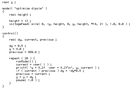
For each pass of the repeat loop, we run the model and compare the latest VSWR that is obtained with a previous VSWR value. If the VSWR is rising instead of falling, we reverse the amount by which we are changing the y value, and we also cut the change step (dy) by half, thus achieving finer and finer adjustments of y as we progress through the repeat loop. y starts at 4.0 and the change in y starts at 0.5.
You can see that the there is a printf statement inside the repeat loop that prints the value of y and the VSWR for that value of y. As mentioned earlier, the output of the printf statement will go into the Output Console of the NC window. The following shows the Output Console after the control loop is done:
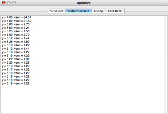
Notice that the minimum VSWR ended up at about 1.22:1. The above example found the lowest VSWR you can achieve with a single center fed straight wire at 14.08 MHz given the default ground parameters in NC and a fixed height for the wire. To get a lower VSWR for the same ground parameters, you could for example include a droop at the ends of the dipole (like with an inverted Vee) as part of the model.
There is a also a pause statement within the repeat loop. This slows the execution down so you that can watch the animation of the VSWR in the Output window. If you are not interested in watching the Output window while the optimization is occurring, you need not include the pause statement and the optimization will run faster.