Smith Chart Interface

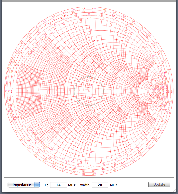
AAplot's Smith Chart interface displays the complex impedance of a test load on a Smith Chart.

A Smith Chart maps the entire right half of a complex plane into a finite circle. AAplot can either plot the measure value as impedance components (resistance and reactance) or as admittance components (conductance and susceptance).

The following figure shows the Smith Chart interface with a chart that is overlaid by a constant 1.5:1 SWR circle.



To get a larger or small chart, resize the AAplot window by dragging the hashed triangle at the bottom right corner the window. You can collapse the Toolbar of the window to obtain a largest possible chart that fits on your computer display. The Toolbar button is the translucent rounded rectangular button at the top right hand corner of the AAplot window.

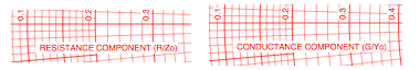
The Impedance/admittance menu lets you switch between impedance or admittance displays. The chart axes labels will switch when you select between the two menu items, for example:



The chart is normalized to the reference impedance that you have chosen (see later). For a 50 ohm reference impedance (Zo), each unit in the impedance scale corresponds to 50 ohms. For example, the point 1+j2 represents a impedance of 50 ohms and inductive reactance of 100 ohms. Similarly, for the same reference impedance (Yo = 1/Zo = 20 milli siemens), each unit of the admittance chart will correspond to 20 milli siemens (milli mhos).

The Fc field lets you select the center frequency of a sweep. The Width field lets you select the width of the sweep (from the lowest to the highest frequency). Readings are taken from the antenna analyzer when the Update button is pressed. A progress bar appears in the space between the Width field and the Update button while measurements are being taken and downloaded.


Smith Chart Options

Smith Chart options are selected in the Smith Chart box in the Parameters window. The window is displayed with the Parameters item in the Window menu of the main Menu Bar.



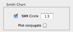
The SWR Circle checkbox and value let you choose to include an SWR circle in the Smith Chart. You can plot the complex conjugates of the data by selecting the Plot conjugate checkbox.

The Zo parameter in the parameters window sets the Smith Chart's reference impedance, which can be complex. All measured values are divided by Zo before being drawn on the chart. For admittance plots, the reciprocal of the normalized result is drawn on the chart. In addition, the data points can be plotted as their complex conjugates by using the Plot conjugate checkbox.

The SWR Circle checkbox determines if you want to overlay a constant SWR circle on the chart. Loads with the same VSWR (referenced to Zo) appear as points that are equidistance from the center of the Smith Chart (i.e., VSWR circles are concentric circles that are centered at the center of the chart). Loads with smaller VSWR will be closer to the center of the Smith Chart and loads that have larger VSWR will be further from the center of the chart.

The SWR Circle text field lets you define the size of the SWR circle. (AAplot ignores SWR circles that are less than 1.05.)

In addition to the parameters in the Post Processing box of the Parameters window, the impedance/admittance menu also does cause the instrument to re-measure data. Until the Update button is again pressed, AAplot reuses the previously measured impedances, but transformed by the new parameters.

The following chart shows a load (a 3m long RG-58 coax cable, terminated at the far end with load that is a 47 ohm resistor in series with a 100 pF capacitor). The sweep is centered at Fc of 24 MHz with a Width of 40 MHz (i.e., a sweep from 4 MHz to 44 MHz).



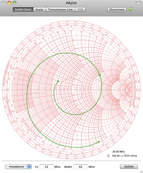
The curve that is drawn is an estimate of impedances for different frequencies, obtained by quadratically interpolating the measured data in the Bilinear transform space.

Notice that one of the plotted green points is a disc that is not completely filled. This is the impedance at Fc and its frequency and impedance are displayed near the bottom right of the window (in this case, 105.43 + j 73.01 ohms).

You can display the frequency and impedance of any other measured data point by clicking along the impedance curve. AAPlot will choose the measurement that is closest to the cursor when the mouse button is clicked, and move the green donut to that measured position and update the data at the bottom right.

The figure below shows the result when a location on the spiral away from Fc is of is clicked.



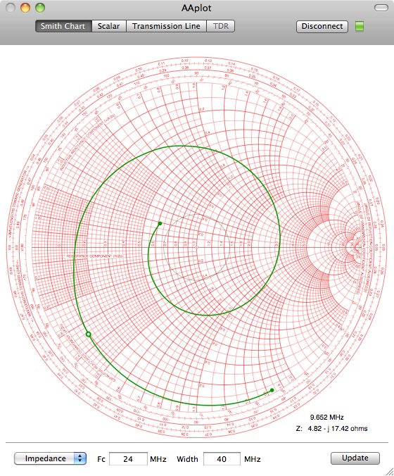
As seen at the lower right corner of the above figure, the frequency of this measured point is 9.652 MHz, with an impedance of 4.82 - j17.42 ohms.

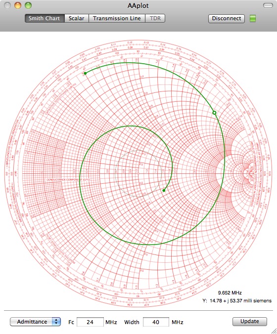
If you change from the impedance plot to an admittance plot (below), notice that the displayed measurement shows up in siemens (mhos).



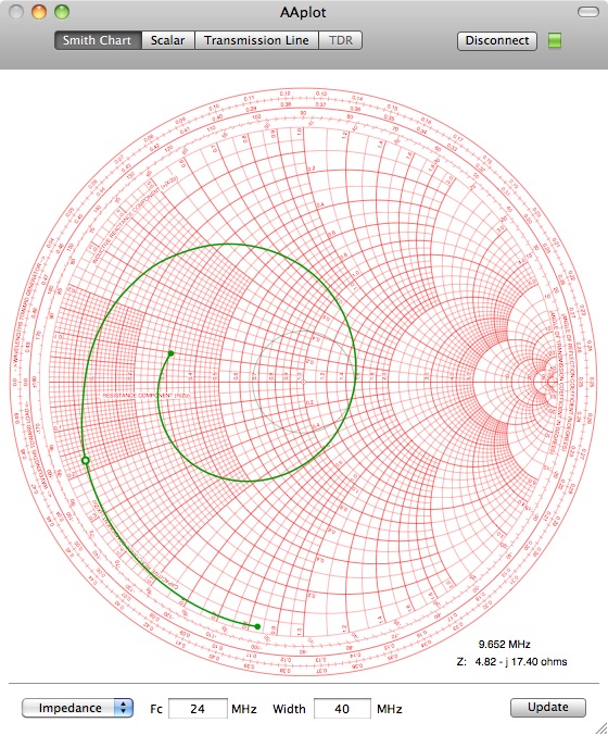
If you change the reference impedance (in the Parameters window) Zo to 100 ohms, the displayed impedance remains the same as the value for Zo of 50 ohms shown in the figure before last. However, the chart is now centered at 100 ohms and take on a different appearance:



You can ask AAplot to use a finer or rougher chart by selecting Fine, Medium and Coarse in the Acquisition Resolution menu. Coarser measurements take less measurement times and is also better on battery life, but may also not be as precise.

You can measure at a single spot frequency either by changing the resolution menu in the Parameters window to Single Frequency, or by zeroing out the width field in the Smith Chart window.

The Timebase Menu in the Smith Chart Parameters window lets you choose between taking a single "One Shot" measurement, or taking continuous measurements.

If you choose either Slow or Fast, AAplot will periodically update the data after you click on the Update button. In the Fast mode, AAplot will start taking the next set of data 0.5 seconds after the last set has finished displaying. In the Slow mode, it will pause for 5 seconds.

With the Fast or Slow trigger modes, the caption of the Update button will change to Stop. Clicking on Stop will break out of the measurement loop after the next data set has finished downloading.