Calibration


AAplot has the capability of calibrating away errors that are introduced by a two-port network that is placed between the bridge of the RigExpert analyzer and the actual impedance that is being measured.

Such a two-port network can be a length of coax transmission line that is connected between the instrument and the feed point of an antenna, or it can be a measurement "fixture" that is built to measure unknown impedances, and can even be errors that are introduced by the SO-239 connector and internal wiring of the antenna analyzer itself.

The correction process used by AAplot follows the "One-port, 3-term Error Model" that is described by D. Rytting of Hewlett-Packard and used in HP and Agilent Network Analyzers.

The calibration process consists of storing measurements of three known impedances for a collection of measured frequencies. AAplot saves the reflection coefficient measurements as calibration profiles in the Application Support folder of your home directory's Library folder. The reflection coefficients in a profile are later interpolated for use at other frequencies when you make measurements of unknown impedances.

As it is usually used, the Rytting calibration is most often performed using three "known" impedances that are (1) a short circuit, (2) an open circuit and (3) a known load resistance that is close to the terminal impedance of the analyzer (e.g., 50 ohms).

However, the bridge topology that is implemented in the Rig Expert antenna analyzers produces very large errors when measuring impedances in regions where the VSWR is large (i.e., when the absolute value of the reflection coefficient is near 1.0). Because of that, AAplot lets you use a moderately low resistance (e.g., 15 to 25 ohms) in place of a short circuit load, and a moderately large resistance (e.g., between 150 to 300 ohms) in place of the open circuit load.

The Calibration Manager item in the Calibration menu in AAplot's main menu bar will open the Calibration Manager's window. The Table View in this window displays the custom profiles for your analyzer that you have measured and saved.



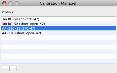
As with all Table Views in Mac OS X, you select the calibration profile to use by clicking on the table view's row. The above figure shows a profile that was named "AA-230 (22-270-47)."

You can unselect all calibrations by clicking on an unoccupied row of the table view.

(The name of the profile that is selected is saved to your plist file so that the next time you launch AAplot, the previous calibration profile, if any, will remain in effect.)

The + and - boxes of the segmented control below the table view let you add new profiles or remove a selected profile.

When the + box is pressed to add a new profile, you will be presented with the calibration window:



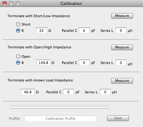
As shown in the figure above, there are three measurements that has to be performed.

One measurement (topmost group) is made by using either a short circuit or a low impedance load.

As mentioned earlier, it is not advisable to choose a true short circuit with a RigExpert analyzer. A "good" value to use is somewhere between 15 ohms and 25 ohms. If the termination has an inductance in series with a resistance and a parallel capacitance across the inductive resistance, you can include those values in the Series L and Parallel C fields.

The second measurement is made with either an open circuit or a high impedance load. Again, as mentioned earlier, because of the circuit topology that is used in RigExpert analyzers, avoid the use of a true open circuit with a RigExpert analyzer. A value of between 150 ohms and 300 ohms works well.

Finally, the third measurement should be made with a resistance that is close to 50 ohms. It does not have to be precisely 50 ohms. However, you do want the three impedance values to be as different from one another as you can construct them, while keeping the VSWR of each load to be no greater than 6.0:1. This will result in the most stable matrix inverses, while also avoiding the places where the RigExpert has the biggest problem with.

You can perform the three measurements in any order.

The progress bar near the bottom of the window shows the progress of a measurement pass. You can abandon a calibration attempt simply by closing the Calibration window when it is not actively measuring (the progress bar is not active).


Profile Names

When all three measurements are completed, the Profile text field and Save button at the bottom of the window will become enabled. You can use any profile name that does not include a / character (the profiles are saved as folders; a / in the folder name will be converted by Mac OS X into something else).

If you decide later to change the name of a profile, you can quit AAplot and go into the AAplot folder in the Application Support folder to change the profile folder's name there. The new name will appear the next time you launch AAplot.

Similarly, you can temporarily remove any currently unused profile from the Application Support folder to reduce clutter of the Calibration Manager window, and move it back in at a later date. The profiles are folders that contain two text files (with measured impedances and target reflection coefficients).

Profiles can be permanently removed by using the - box in the Calibration Manager window.


Reference Loads

For the HF region, the reference loads can be constructed using ordinary non-inductive resistors. I find that garden variety 1/8 watt 2% axial resistors work quite well. I construct my load inside the body of a PL-259 coax plug. One end of the resistor is threaded through and soldered to the coax connector's center pin and the other end of the resistor is bent back and fed out through one of the solder holes of the plug and soldered to the body of the plug. Keep the leads short and keep the body of the resistor away from the inside wall of the plug.

Measure the actual resistance with a good DVM and use that as the resistance of the load. This should be sufficient for non-critical measurements in the HF region.


Example 1 -- Calibrated analyzer vs Uncalibrated analyzer

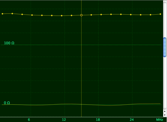
The following shows the measurement done on an uncalibrated AA-230PRO. A 150 ohm resistor that is mounted inside a PL-259 plug is connected directly to the SO239 connector on the analyzer:



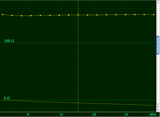
The solid yellow line is the resistive component and the dotted yellow line is the reactive component of the measured impedance.

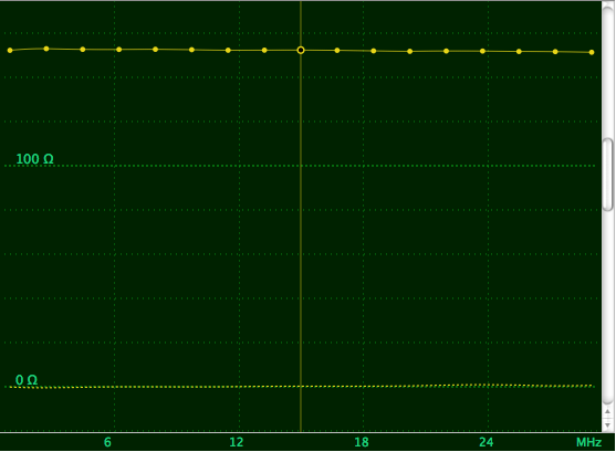
The following shows the corrected measurement of the same load. The calibration profile is constructed by inserting the three calibrating loads (22.0 ohms, 271.2 ohms and 46.8 ohms) that are inserted directly at the AA-230PRO's SO-239 connector.





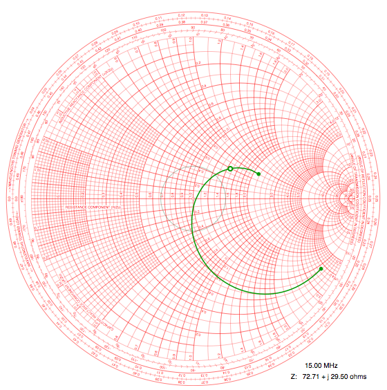
Example 2 -- Calibrated coax cable with a known resistive load

The following shows the measured impedance of a 3m length of RG-58 cable that is terminated by the same 150 ohm resistor above. The frequency is swept from 1 MHz to 29 MHz:



The typical constant SWR arc that is formed by typical short length (thus low loss) of transmission line is easiiy recognized. The SWR circle is centered at the characteristic impedance of the coax cable, which can be seen to be a tad off from 50.0 ohms for the Smith Chart center.

A calibration profile is created for this 3m cable by calibrating it with the same 22 ohm/270 ohm/47 ohm set of load resistors that was used earlier.

The following shows the output when the 3m cable that is terminated with the fixed 150 ohm load is measured with the calibration profile for the cable:



Notice that the corrected measurements are so close to a single value that they all fell inside (and under) the green donut. The cable has been calibrated away and practically disappeared. The Scalar plot looks like this:





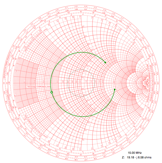
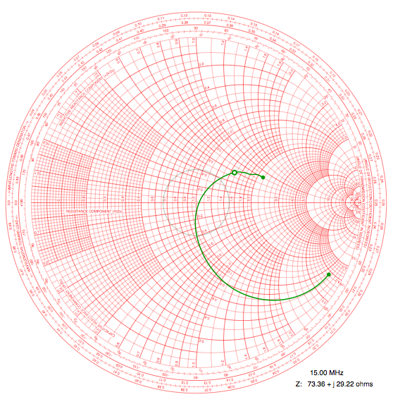
Example 3 -- Calibrated coax cable with a complex load

The following shows the uncalibrated Smith chart for an artificial complex impedance that is made up of a resistor, an inductor and a capacitor all in series. (The load was constructed to be close to resonant and near 50 ohms at the low end of the 40m Amateur band.) The load is plugged directly into the SO-239 connector of the AA-230PRO:



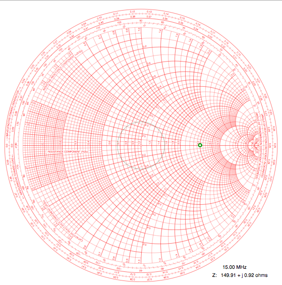
When this complex load is use to terminate the same 3m RG-58 that is used in Example 2 above, the uncalibrated output of the AA-230PRO shows this:



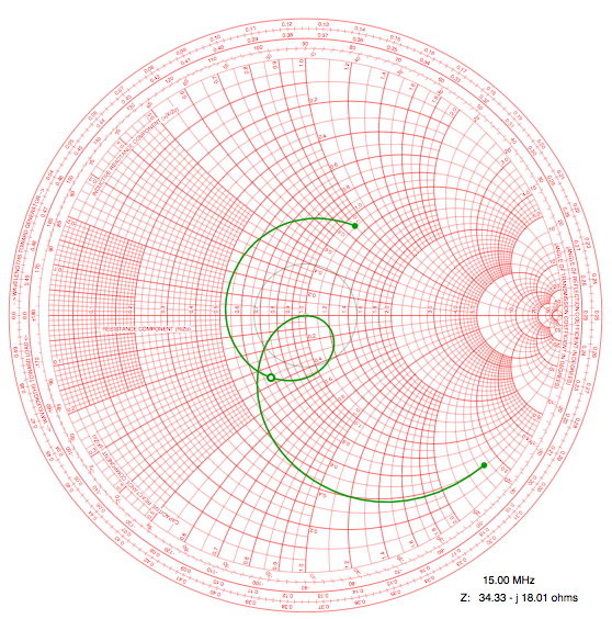
Notice that this bears very little resemblance to the actual impedance sweep that is shown in the previous Smith Chart.

We now apply the 3m coax cable profile that was used in Example 2, and the corrected measurement shows:



There is some error at the higher frequencies. Overall however, the result is quite close to the measurement of the complex load directly at the analyzer's connector.