
cocoaPath - Technical and Implementation Details
Kok Chen W7AY [w7ay
(at) arrl . net]
Last updated: August 27, 2008
1 Introduction
cocoaPath uses the ionospheric
propagation model that is based on the paper "Experimental Confirmation of an HF
Channel Model" by Clark Watterson, John Juroshek and
William Bensema which was published in the December 1970
issue of the IEEE Transactions on Communication
Technology (henceforth called the "Watterson model").
The Watterson model has been widely adopted, including by
the ITU-R F.1487 recommendation
(henceforth referred as the "ITU" document) and the
CCIR 520-2 recommendation (henceforth
referred to as the "CCIR" document) which the ITU
document supersedes.
This section of the cocoaPath documentation discusses the
internal workings of the program.
2 The
Watterson HF Channel Model
The Watterson model consists of a signal that is reflected
by the ionosphere into multiple signal paths.
Each path consists of either a single magneto-ionic
component, or two such components that are split from one
another by a Doppler frequency shift. Each
magneto-ionic component is then modulated by an independent
scattering function. The
scattering function is a complex valued random process that has both a
Gaussian spectrum and a Gaussian
amplitude distribution.
The following figure (taken from the ITU recommendation; it
also appears in the original Watterson paper) shows the two
components of a single path.
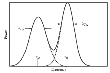
Figure 2-1 Two-Component
Watterson Path
Under most circumstances, as
mentioned in the ITU document, we only need to include
paths with a single component, shown in Figure 2-2 below.
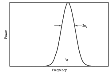
Figure 2-2
Single-Component Watterson Path
Because the Watterson model is
linear, we can replace a path that has two components by
two separate single-component paths that share an identical
time delay.
Even though each path in cocoaPath has only a single
component (like that shown in Figure 2-2), all paths in
cocoaPath can share the same time delay. Two-component
paths can therefore be modeled in cocoaPath by using two
different paths that share the same time delay, with each
path using a different Doppler shift to model the
magneto-ionic split that is shown in Figure 2-1 above.
(Note: all the models that are specified in the ITU
document consist of two paths; each path having only a
single component with no magneto-ionic splitting.)
Each scattering function is a complex valued random
variable with zero mean Gaussian statistics and Gaussian
passband centered at DC. The passband width is defined by a
frequency spread parameter. As seen in Figures 2-1 and 2-2
above, the frequency spread is defined by the points on the
Gaussian curve that are separated by two standard
deviations of the probability density function (the
standard deviation is commonly known by "sigma"), and have
a two-sigma value of between 0.1 Hz to 40 Hz.
This complex valued scattering function modulates an input
signal that represents a complex signal with in-phase and
quadrature terms. For the case where a two-component model
is needed, the center of the Gaussian passband is shifted
by the Doppler shift frequency by multiplying the signal
with a complex phasor.
Depending upon the precise propagation condition, a signal
that takes multiple ionospheric paths can arrive at
different times. This results in differential time
delays between the various paths of up to 20
milliseconds.
The outputs of the scattered paths are summed to form the
final output signal. The following figure shows a Watterson
model that has two paths, with a delay line to provide the
time delayed signal of a path. The delay line is fed from
the in-phase and quadrature terms of the input scalar
valued signal that has been Hilbert transformed. A Hilbert
transform is basically a broadband 90-degree phase shifter.
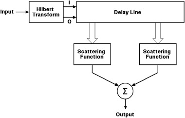
Figure 2-3 Two-Path
Watterson Model
As described above, a Watterson
path that has two magneto-ionic components can be modeled
as shown in Figure 2-4. Notice that two scattering
functions are applied to the same delay line tap. In this
case, the two scattering functions would each have a
different Doppler shift frequency.
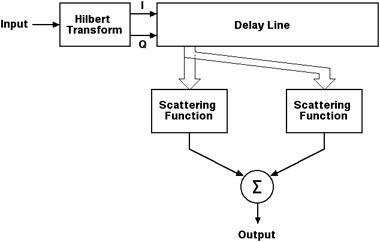
Figure 2-4 Implementation
of a Single-Path Watterson Model with Two Magneto-ionic
Components
Note that the time delay of the
Watterson model is stationary in time since the model
implements each time delay as a discrete tap of a delay
line. If better models are needed, an easy modification can
be made to cocoaPath to implement continuous time-varying
delays by taking multiple delay line taps from a
neighborhood in the delay line and weighting them with time
varying coefficients.
3 In-phase
and Quadrature Delay Line
As shown in Figure 2-3 of the previous section, a scalar
input signal from a sound source is first converted by a
Hilbert transform into an analytic signal which has an in-phase
(I) and a quadrature (Q) term. This is done so that the
complex version of the input signal can be modulated by
a complex valued scattering function. The Hilbert
transform also limits the passband of the input signal.
cocoaPath allows you to select from bandwidths of 1.24
kHz, 3 kHz and 4 kHz.
The Hilbert transform is designed by starting with a
511-tap lowpass FIR filter whose bandwidth is a half of the
bandwidth of the desired Hilbert transform, fB. The impulse
response of this FIR filter is an appropriate sinc function that is multiplied by a
Blackman-Harris window. The prototype
lowpass filter is then translated by multiplying the
impulse response with a sinusoid at (fB/2+100) Hz - the
result is a bandpass filter that extends from 100 Hz to
(fB+100) Hz.
The impulse response of the in-phase bandpass filter is the
impulse response of the prototype lowpass that is
multiplied by a cosine function at fB/2+100 Hz and the
impulse response of the quadrature bandpass filter is the
impulse response of the prototype lowpass filter that is
multiplied by a sine function at fB/2+100 Hz. The impulse
response of the in-phase filter can be seen as part of
Figure 3-4 below.
Figure 3-1 shows the magnitude response of the in-phase
(red) and quadrature (blue) filters of the Hilbert
transform section. The filters shown are designed to be
3000 Hz wide between the -3 dB points. The horizontal grid
lines shown are separated by 10 dB. It can be seen in the
figure below that the first sidelobe of the Blackman-Harris
windowed filter is 65 dB below the passband response. Any
significant mismatch between the in-phase and quadrature
terms are also at those low levels.
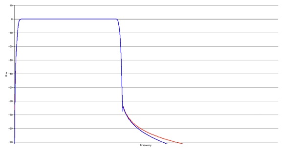
Fig 3-1 Hilbert Transform
Magnitude Response (red = in-Phase, blue =
Quadrature)
Figure 3-2 shows the phase
difference between the in-phase and quadrature channels for
the filters whose magnitude responses appear in Figure 3-1.
The vertical axis ranges from 89 degrees to 91 degrees.
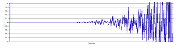
Fig 3-2 Hilbert Transform
Phase Difference (89 to 91 degrees)
The following figure is the same plot as Figure 3-2, but
with the vertical axis expanded to display between 89.9999
degrees and 90.0001 degrees:
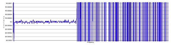
Fig 3-2 Hilbert Transform
Phase Difference (89.9999 to 90.0001 degrees)
The peak phase deviation from a perfect 90 degree
quadrature is 2.5 milli-degrees for any part of
the passband that is above -60dB of the full scale
magnitude.
As shown in the earlier block diagram (Figure 2-3), the
in-phase and quadrature components of the input signal are
passed through a two channel delay-line. An appropriate tap
of this delay line provides the time delayed signal for a
Watterson path. Figure 3-4 shows the impulse response of
the in-phase filter at two different taps (red and blue
plots) of the delay line that are separated by 8
millseconds.
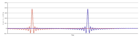
Fig 3-4 Delay Impulse
Response (8 ms)
The delay line in cocoaPath is
implemented with a floating point ring buffer that is 128
milliseconds long. The signal is processed in blocks of 32
milliseconds, thus cocoaPath allows models that have
differential path delays of up to 96 milliseconds.
cocoaPath uses a processing sampling rate of 16,000 samples
per second, so the delay line has a resolution of 0.0625 of
a millisecond. ITU suggests using a time delay of up to 20
ms, with a resolution of up to 0.5 milliseconds.
In addition to storing both the in-phase and quadrature
signal pair, the delay line in cocoaPath is actually twice
the length of a basic ring buffer, the second half being an
identical copy of the first half. When an input sample
arrives, it is inserted into both halves of the double
length ring buffer. This allows subsequent scattering
functions to treat a delay line pointer as a contiguous
block of data, without having to deal with the wrap-around
nature of a normal ring buffer.
4 The
Watterson Scattering Function
A general
Watterson model consists of multiple signal paths, each
path having a different time delay parameter. Each path can
consist of up to two magneto-ionic components that are
separated by a Doppler shift. However, as mentioned in
Section 2, it is sufficient to implement single-component
Watterson paths. A multi-component path can be created as
two separate paths that are tapped off the same location in
the delay line, but having different Doppler shifts.
According to Figure 2-2, a single-component path is defined
by three scattering parameters consisting of the path
attenuation, the frequency spread and the Doppler shift.
The attenuation determines the amplitude of the Gaussian
function, the frequency spread is defined by twice the
standard deviation of the Gaussian and the frequency shift
is defined by the horizontal displacement of the mean of
the Gaussian along the horizontal axis.
The attenuation is implemented by multiplying the signal by
a scalar constant. The scattering function is implemented
by multiplying ("modulating") the signal by a Gaussian
random variable, and the Doppler frequency shift is
implemented by multiplying the signal by constant amplitude
phasor.
Since these three operations are linear, they can be
performed in any order. Furthermore, since we only need a
scalar signal for the output stream, the attenuation term
can be applied to the scalar output instead of to the
analytic signal.
Figure 4-1 shows the scattering function as implemented in
cocoaPath, first applying the Doppler frequency shift by
multiplying with a complex phasor (a sine/cosine oscillator
pair) , then multiplying the delayed in-phase and
quadrature input signal by a complex signal source that is
a Gaussian random process, and finally
extracting a scalar signal from the analytic signal and
applying a gain factor to implement the attenuation term
of the spreading function.
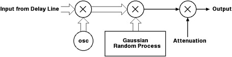
Figure 4-1 Scattering
Function
4.1 The
Gaussian Random Process
The Gaussian scattering function is central to
the Watterson model.
The Watterson scattering function consists of two (i.e.,
in-phase and quadrature) independent Gaussian random
variables. Mathematically, they form a vector which has a
bivariate Gaussian distribution. The
modulus of a complex variable from an independent
bivariate Gaussian random process is known to have a
Rayleigh distribution. This is why a
Gaussian scattering function produces the familiar
Rayleigh fading that is encountered
in HF propagation.
The Gaussian process in the Watterson model has a Gaussian
distribution both in amplitude and in frequency. cocoaPath
starts by generating a pair of random Gaussian number
streams. The two random streams are then pass through two
filters that have an identical Gaussian frequency response.
For each of the in-phase and quadrature components,
cocoaPath starts by using the using the Wichmann-Hill method to generate a
white, uniform distribution noise The
uniformly distributed noise is then passed through the
cartesian form of the Box-Muller method to create a white,
Gaussian distributed noise.
The white noise from the Box-Muller algorithm is passed
through a filter which has a Gaussian bandpass profile. The result
is a random process that has a Gaussian distribution
both in time and in frequency.
The Gaussian filter is created by cascading identical
simple FIR filters. Each simple FIR filter
has 6 equally weighted taps, forming a rectangular
impulse response. A cascade of 227 of these simple
filters creates an equivalent 1361-tap FIR filter which,
by the Central Limit Theorem, produces an
impulse response that approximates a Gaussian. Since the
Fourier Transform of a Gausssian is yet
another Gaussian, the frequency response of this
1361-tap FIR therefore has a passband which approximates
a Gaussian.
Figure 4-2 shows the frequency response |H(ƒ)| of the
cascaded filter (in red) and the error (in dotted blue
line, and scaled by a factor of 1000) when compared to a
true Gaussian of 197.81 Hz bandwidth. The Central Limit
Theorem works particularly well; the peak error shown in
the figure below has a deviation of less than -50 dB full
scale.
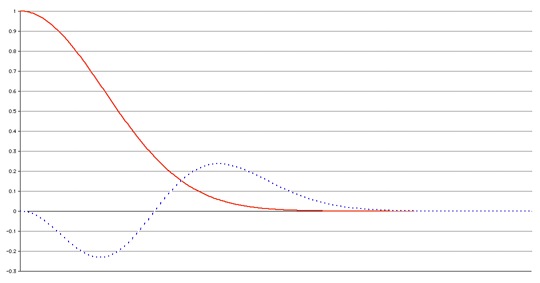
Figure 4-2 Gaussian
Approximation and Error (x1000)
Figure 4-3 shows the same filter in the log scale (red)
with the true Gaussian passband (in a dashed white-blue
line) down to -90 dB of full scale.
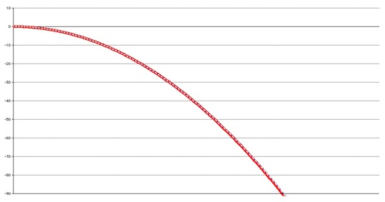
Figure 4-3 Gaussian
Approximation (dB) vs actual Gaussian Filter
The above Gaussian filter operates at a fixed bandwidth. To
obtain the 0.1 Hz to 40 Hz spreading bandwidths that is
required by the ITU recommendations, the random values from
the Gaussian filter are up-sampled using the Audio Converter routines in Mac OS
X's Core Audio framework .
Audio Converter can resample between arbitrary sampling
rates, however it can only be used for a limited range.
cocoaPath solves this by up-sampling in multiple steps, the
first steps use Audio Converter to resample by a power of 2
and the final step uses Audio Converter to resample by an
arbitrary ratio. A 1 Hz spreading filter is created from
the 198 Hz wide signal by up-sampling with a factor of 16
and then with a factor of 12.36. A 0.1 Hz spreading filter
is created by first up-sampling with a factor of 8, then by
a factor of 16 and finally by a factor of 15.45.
The transition band of the interpolation
filter in the Audio Converter creates an error of
approximately 0.2% and this is compensated by increasing
the noise power by a corresponding amount.
The result of the pair of in-phase and quadrature noise
generators and Gaussian filters is a bivariate Gaussian
process whose magnitude is 1.0.
5 Additive
White Gaussian Noise (AWGN)
The
Watterson model introduces Gaussian random processes to
scatter the paths without adding noise to the amplitude of
the signal. The ITU document recommends adding band-limited
Gaussian noise to the output of the model to set the
signal-to-noise ratio.
cocoaPath generates a wide bandwidth Gaussian noise using
the same Wichmann-Hill and Box-Muller generators that it
uses for the Doppler scattering function (see section 4.1
above). The samples from the Box-Muller algorithm are
treated as scalar values by making the complex value pairs
into two successive independent scalar Gaussian samples.
The noise samples are then pass through a bandpass filter
that is identical to one channel of the bandpass filter
used in the Hilbert transform which was mentioned in
section 3 above. This scalar noise is then added to the
scalar output from the Watterson model.
As in the Hilbert transform, the bandwidth of this filter
can be chosen from 1.24 kHz, 3 kHz or 4 kHz. The filter
starts at about 100 Hz and, in the case of the 3 kHz
filter, extends to 3100 Hz. The result is noise that is
"white" within the passband of the selected filter.
As shown in Figure 5.1 below, the RMS noise power in set
with the AWGN text field of the cocoaPath user interface
(relative to a digitized "full-scale" signal). When an
input signal appears, cocoaPath will compute the noise
power from the input source and display the signal-to-noise
ratio.
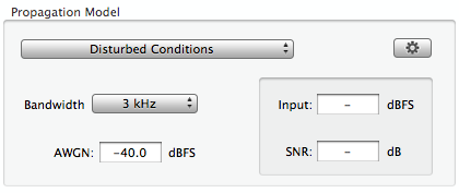
Figure 5-1 Noise and
signal-to-noise parameters
The RMS power from the model
(before white noise is added) is computed by passing the
input signal through an equivalent multiple path Watterson
model, but with the Doppler scattering suppressed. This
ensures that there is no fluctuation in the power
computation, while taking into account what the different
paths in a model can do to a signal (paths can
constructively or destructively interfere with one
another). Since the mean gain of a Doppler spreading
function is unity, the power from a model that has no
Doppler spread should be the same as the long term mean RMS
power of the signal that includes Doppler spreading.