Kok Chen, W7AY
w7ay (at) arrl (dot) net
December 16, 2012

[This is the second revision of the article which I first wrote in 2008 (an earlier revision was mostly a cosmetic update). This expanded revision includes references and additional details and diagrams to explain the underlying principles. A discussion on how this ATC pertains to Leonard Kahn's "Ratio Squarer" is included in this revision, together with a comparison of error rates. Section 4 is added to show an improvement over the traditional ATC by applying only the clipper from the optimal ATC. The previous version of this manuscript is available here.]


1. Introduction

Automatic Threshold Correction (ATC) is a technique that is used in frequency shift keyed (FSK) reception to optimize the decision threshold level in the presence of selective fading.

On-Off Keying (OOK) was used in early wireless transmission of teletype data. With OOK, a single carrier is keyed on and off to convey binary information. However, Rayleigh fading on HF propagation channels causes loss of data when the narrow band OOK signal fades close to the noise floor.

Frequency Shift Keying (FSK) keys two separate carriers in a complementary manner. When one carrier is turned off, the other carrier is turned on. One of the carriers of FSK is called the Mark carrier, and the other carrier is called the Space carrier. The separation of the carriers is called the FSK “shift.”

In an Additive White Gaussian Noise (AWGN) channel, FSK has a 3 dB sensitivity advantage over OOK when both of transmitters use the same peak power. The two toned FSK signal is substantially superior to OOK since it also provides a form of frequency diversity. When a multi-path signal produces selective fading, one of the two carriers can survive sufficiently for the FSK signal to still be decoded without errors when the other carrier has faded completely away.

The ATC is a circuit, or an algorithm in the case of a software modem, that determines how the Mark and Space tones are combined to take advantage of their behavior during selective fading. An implementation of DC restoration (often called an accessor in early papers) which provides the foundation for early ATC development was described as early as 1948 in Sprague's '434 patent [reference 1].

This article introduces two new ATC schemes that improves upon the "traditional" ATC. Section 4 shows that under fading, the inclusion of a simple clipper can add about 0.5 dB of sensitivity compared to the traditional ATC, while the fully optimized ATC that is described in Section 6 can improve the sensitivity by about 1 dB compared to the traditional ATC.


2. FSK Demodulation

In the simplest form, shown in Figure 2.1, the information bits from an FSK signal are demodulated by subtracting the amplitude of the detected Space component from the amplitude of the detected Mark component. When the difference is greater than zero (the threshold level), a Mark is assumed to be sent. If the difference is less than zero, a Space is assumed to be sent. This process of transforming an FSK waveform into a binary level is often called slicing.

Figure 2.1: Simple FSK Demodulator

The Mark and Space filters in Figure 2.1 are bandpass filters that are centered on the Mark and Space frequencies respectively. For an unbiased slicer, both filters are designed to have identical noise bandwidth.

The detectors of an FSK demodulator can also operate on baseband signals, as illustrated in Figure 2.2.

Figure 2.2: Baseband FSK Demodulator

With the baseband approach, the input signal is mixed by Mark and Space local oscillators into two baseband signals, which are then filtered by identical lowpass filters. The baseband approach is easily adaptable to moving Mark and Space frequencies, without needing to change data filters. Different data filters are still needed when the baud rate changes.

The mixers in Figure 2.2 can also be implemented as quadrature mixers which produce baseband outputs that are analytic. After passing through complex data filters, the detectors can be precisely implemented by taking the moduli of the filtered components. The quadrature mixed baseband approach is often used to implement software FSK demodulators since the detector is close to being ideal.

For optimal demodulation of an FSK bit stream under AWGN, a Matched Filter is used for the aforementioned filters.

Matched filters for rectangular pulses are spectrally wide and susceptible to interference by an adjacent signal. For this reason, the filters in Figure 2.1 are often implemented with narrow bandpass filters, or in the case of the baseband approach in Figure 2.2, by narrow lowpass filters.

To avoid inter-symbol interference (ISI), the narrower filters can be designed to satisfy the Nyquist criteria [reference 2, 3]. (An FSK Matched Filter, by its definition, satisfies the Nyquist criteria.) In practice, one needs to balance the need to reduce of ISI with the need to reject adjacent channel interference and reducing in-band noise.

The narrowest Nyquist filter for a rectangular pulse under AWGN is the Raised Cosine filter. Although a Raised Cosine filter generates no internal ISI, its performance is slightly poorer than a Matched Filter, which accepts more energy from the FSK signal. See here for a family of filters with increasing bandwidths, starting with the bandwidth of the Raised Cosine and in the limit, ending with the bandwidth of a Matched Filter, with corresponding better FSK decoding as the bandwidth is increased.

Another factor that affects the choice of filter bandwidth is that the HF channel can widen the transmitted pulse width, causing large errors from a Raised Cosine that is designed for a perfect pulse.

For an ideal FSK signal with baud rate B, the 6 dB cutoff for a Raised Cosine filter is B/2 Hz, with zero response past B Hz. The impulse response of a Raised Cosine filter therefore rings indefinitely. When a Raised Cosine filter is approximated with an FIR structure, the Raised Cosine impulse response is truncated to have a finite support and thus, like all FIR filters, cannot be truly bounded in the frequency domain.


3. Automatic Threshold Correction (ATC)

Selective fading causes the Mark and Space amplitudes to become unequal. When that occurs, the simple FSK demodulators with the unbiased thresholds are no longer optimal. Frerking [reference 4] has a detailed analysis of an Automatic Threshold Correction (ATC) circuit when the Mark component of an FSK signal suffers a deep fade.

The standard ATC circuit, shown in Figure 3.1, is created by adding a pair of envelope detectors (shown in the figure below as boxes labelled ENV) to bias the levels of the detected Mark and Space signals. The envelope detector tracks the amplitude of a carrier as it goes through a fade. In the simplest implementation (the one described in Frerking), the envelope detector can be a simple Fast-Charge-Slow-Discharge circuit (most often seen in AGC circuits). The time constants are chosen to be slow enough so that the ENV output does not track individual data bits.

With a software demodulator, it is very easy to delay the actual signal path relative to the ENV path so the ENV stage can look ahead at the “future” trend of the envelope. With a lag of just a dozen bits, much better estimates of the Mark and Space envelopes can be obtained compared to the use of Fast-Charge-Slow-Discharge circuits.

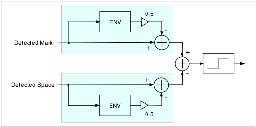
Figure 3.1: Automatic Threshold Correction (ATC)

As seen in the above figure, one half of the envelope is subtracted from the input signal. When the two FSK carriers no longer have equal amplitudes, the two envelopes become unequal and that in turn biases the slicer threshold towards the midpoint of the Mark and Space envelopes.

Since the incoming detected Mark and detected Space signals also includes detected noise (not zero mean), the ATC as described above is still not completely unbiased when the noise term is non-zero.


4. Compensating for the Noise Floor

With a little extra complexity added to the linear ATC that was shown in Figure 3.1, we can account for a non-zero noise floor.

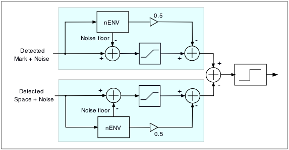
Figure 4.1: ATC with Noise Floor Correction

In Figure 4.1 above, in addition to the envelope, the noise floor is also computed in the nENV stages shown. The noise floor is subtracted from the signal itself.

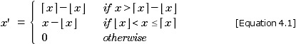
After removing the noise floor, the signal is sent to a clipper that prevents the translated signal from falling below zero in case the instantaneous signal falls below the average noise floor. The clipper also keeps the output from exceeding the value of the envelope (ceiling), viz.



Since the composite envelope also includes a noise contribution, the same noise floor has to also be subtracted in a similar manner from the composite envelope to maintain an unbiased threshold.



Because the same amounts are subtracted from both Mark and Space channels, the noise floor adjustment has no effect when it is not used in conjunction with a clipper. The combination of noise subtraction and clipping is surprisingly effective; this clipped ATC can, for example, improve demodulation sensitivity of the traditional ATC by 0.5 dB, and reducing error rates by about a factor of two, when one carrier is 10 dB weaker than the other (see charts in Section 7 below).

If the Mark and Space filters have identical noise bandwidth, a slight improvement can be realized by averaging the noise power that are measured by the two nENV stages and using the mean as the common noise power for both Mark and Space correction.


5. An ATC Problem

The ATC automatically turns the demodulator into a Mark-only demodulator when the Space signal fades completely away, and it automatically turns the demodulator into a Space-only demodulator when the Mark signal fades completely away.

In between these two extremes, and different selective fading ratios, the ATC that is shown in Figure 3.1 establishes an unbiased threshold for the slicer to compensate for the difference in the amplitudes of the Mark and the Space signals.

A closer inspection shows however that there is a problem with the ATC circuit shown. While the decision threshold may be optimal, the signal to noise ratio (SNR) is not. I had serendipitously stumbled upon this while investigating better methods for estimating the Mark and Space envelopes.

Notice that even when multipath causes the Space signal to completely fade away, the noise (combination of sky noise and receiver noise) from the Space filter survives, and the ATC circuit can be reduced to Figure 5.1 below.

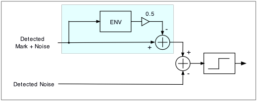
Figure 5.1: ATC Under Mark-only Condition

The decision threshold for the slicer remains correct, assuming that the Mark and Space filters both have the same noise bandwidths. Since noise is uncorrelated with the Mark signal, the "Detected Mark + Noise" term can be written as "Detected Mark + Detected Noise."

Compare the above figure to a true Mark-only demodulator, shown in Figure 5.2.

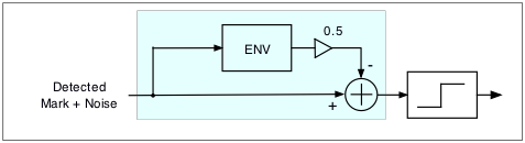
Figure 5.2: Mark-only Demodulation

Since the noise contribution from the Space channel remains in the ATC circuit (Figure 5.1), the slicer sees about 3 dB more noise than the slicer in the Mark-only circuit (Figure 5.2).

Because of this, the traditional FSK demodulator (with or without an ATC) will have a degraded signal to noise ratio even when one of the channels has only partially faded away, reaching a 3 dB deficit in SNR when one of the carriers has faded completely away.


6. SNR-optimized FSK Demodulator for Selectively Fading Channels

We can attempt to remove the noise contribution from a channel that is under selective fading by applying a controlled gain term before the faded signal reaches the slicer. Figure 6.1 illustrates a gain controlled stage in the Space path case where an ATC is not used. The magenta region models the Space signal with a fade factor of k.

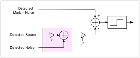
Figure 6.1: Fading Model

Given uncorrelated noise in the Mark and Space channels, and a selectively faded Space signal that is attenuated by a factor k relative to the Mark signal, the SNR at the slicer is proportional to



where µ is a gain that is applied to the Space path. The numerator is proportional to the total signal power as seen by the slicer, while the denominator is proportional to the total noise power.

By setting the derivative of Equation 6.1 with respect to µ to zero, it can be seen that the maximum SNR is achieved by making µ = k, viz. to optimize SNR, µ should be linearly proportional to the fading factor k.

Recall that the ENV (envelope detector) stage measures a scalar that is proportional to k , Figure 6.2 shows the ATC-less FSK demodulator that optimizes the SNR for the slicer when there is selective fading from either Mark or Space signals (by superposition, the same Equation 1 applies to the Mark channel).

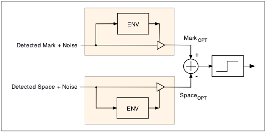
Figure 6.2: ATC-less Demodulator that is Optimized for Selective Fading

The ATC bias for Mark_OPT and Space_OPT in Figure 6.2 can be derived per Frerking, e.g., the bias for Mark_OPT is one half of ENV(Mark_OPT). It can also be seen by inspection that ENV( x.ENV(x)) is just ENV²(x).

By including the ATC component to Figure 6.2, we get the FSK ATC that is optimized for a selective fading that is shown in Figure 6.3.

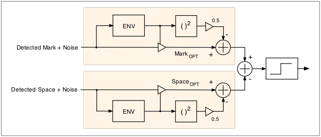
Figure 6.3: FSK Demodulator that is Optimized for Selective Fading

Notice that the mark and space filter outputs in the above figure are multiplied by a gain factor before they are sliced. As we had mentioned earlier, the optimal gain is achieved by multiplying the mark and space signals by the amplitude of their own envelopes. Thus the gain control terms are simply the output from the envelope detectors.

When the envelope of a channel drops by a factor of k, for optimal SNR, we attenuate it further by yet another factor of k. Thus, a channel that has selectively faded by a factor of k will move the optimal slicer threshold (the rightmost parts of the shaded areas in the above figure) by a factor of one half of the square of k.

With this algorithm, when the Space signal fades all the way down to the noise floor due to selective fading, the output of the space filter (which includes the noise in the Space channel) is reduced to zero before is subtracted from the Mark signal. As a result, the noise from the space filter is also attenuated to zero. I.e., during extremely deep selective fading, this new demodulator behaves precisely like a Mark-only demodulator that was shown in Figure 5.2.

Finally, by incorporating the noise floor compensation and clipper that was shown earlier in Figure 4.1, Figure 6.4 shows the FSK ATC that is optimized for selective fading and noise floor.

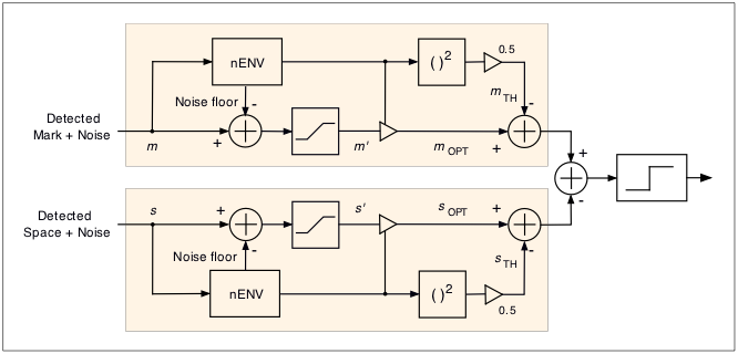
Figure 6.4: FSK Demodulator that is Optimized for Selective Fading (Noise Compensated)

Following Figure 6.4, if we let m and s be the detected Mark and Space signals (including noise), and n be the common noise floor, then



and



The slow control signals that are generated by the nENV stages are defined as



and



where env(m) and env(s) are the envelopes of the detected Mark and Space signals (that includes noise).

The SNR optimized Mark and Space signals are thus:



and



while the threshold bias values are



and



The demodulator then determines that a Mark is received if



otherwise, the demodulator determines that a Space is received.


7. Performance

The following is a plot of Character Error Rate (CER in percentage of character errors) versus signal-to-noise ratio (SNR) for a 45.45 baud start-stop FSK signal in an AWGN channel where the Mark and Space carriers are imbalanced by 10 dB (to simulate sustained selective fading where one of the carriers has faded by 10 dB).

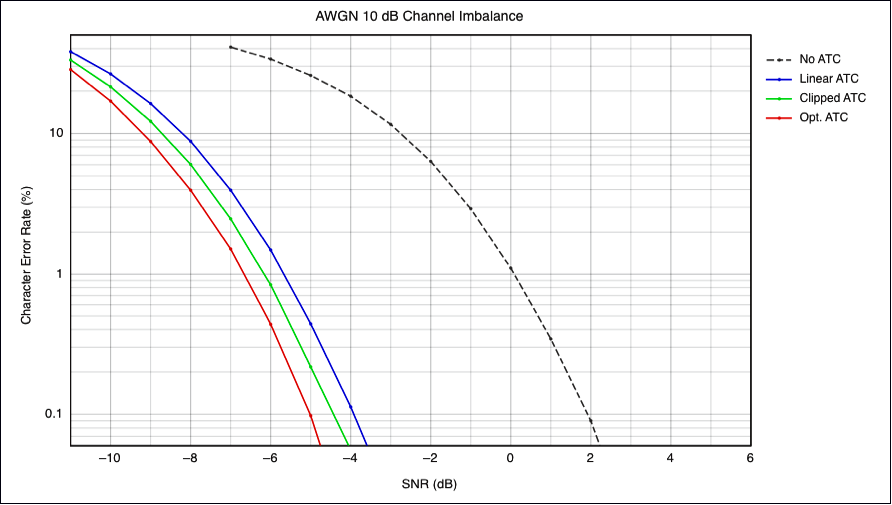
Figure 7.1: ATC Performance with 10 dB Channel Imbalance

The SNR (horizontal axis) is referenced to a noise bandwidth of 3 kHz. For the SNR in a 300 Hz noise bandwidth, add 10 dB to the horizontal scale.

The black dashed curve is the error rate in the absence of an ATC circuit. The blue curve is for a traditional "linear" ATC, as described in Section 3. The green curve is for the ATC with a clipper that is described Section 4. The red curve is for the SNR optimized ATC that is shown in Figure 6.4 of Section 6.

(Please note that the previous version of this article had used synchronous bit clocking. The error rate for chart above is computed using asynchronous 5 bit characters, with 1 start bit and 1 stop bit).


8. Conclusion

It can be seen from Figure 7.1 that for a 2% character error rate and given a 10 dB Mark/Space imbalance, a simple "linear" ATC improves sensitivity of a demodulator that has no ATC by about 5.7 dB. An extra 0.5 dB is gained by introducing a clipper into the ATC correction signal.

The SNR-optimized ATC gains yet another 0.5 dB to produce a total of approximately 1 dB improvement over the linear ATC.

It can also be seen that under the above conditions, the optimized ATC produces 3 times fewer error than the linear ATC when the SNR is -6 dB.


Appendix A: Kahn's Ratio Squarer

Leonard Kahn applied for a U.S. patent in 1953 for a method to combine the outputs from diversity receivers. The patent was granted U.S. Patent 3,030,503 in 1962. Kahn also submitted a correspondence ("Ratio Squarer") to the Proceedings of the IRE in 1954 that described the same method [Reference 5].

Until Kahn's work, the primary method for diversity reception was to pick the stronger signal from two diversity receivers. Kahn instead suggested summing the output from the receivers after applying a correction to optimize the SNR of the resulting sum.

Kahn had started with (the following equations are taken from Kahn's papers):



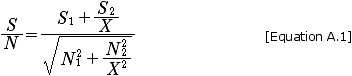
as the SNR of the sum of the outputs from the two individual receivers, where X is the ratio that is applied to the output of receiver 2 before it is added to the output of receiver 1. S₁/N₁ and S₂/N₂ are the SNR at the two receivers. When N₁ = N₂ (i.e., the two receivers have the same noise bandwidth), Kahn determined that for optimal SNR,



which leads to Kahn's "Ratio Squarer" equation,



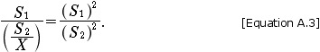
I.e., the optimal way to directly combine the signals is to take the square (power) from each receiver. Please note that implicit in this result is the need for the noise bandwidths of the two receivers to be identical.

When selective fading causes only one of the FSK carriers to fade, the Mark and Space carriers can be considered to be components of a frequency diversity system. For this reason, the Kahn "Ratio Squarer" has been used in FSK demodulation to square the detected Mark and detected Space signals before submitting the Mark and Space powers to a slicer.

Note that squaring the Mark and Space signals is different from the approach that was describe earlier in Section 6. The method that was described in Section 6 applies a slowly varying gain adjustment to a scalar value (e.g., the detected Mark signal). After being gain controlled, the values that are sent to the slicer remain as scalars. By following Kahn, the squaring of the detected Mark and Space signals results in the slicer working on powers instead of on scalars.

Figure A.1 below shows the result when the squared signals are passed through an ATC that works on power values (green curve). Interestingly, the use of a clipper from Section 4 also improves the performance of the squaring demodulator (red curve).

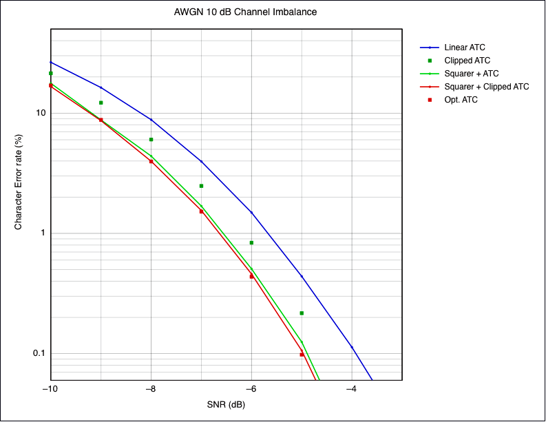
Figure A.1: Squarer + ATC Performance with 10 dB Channel Imbalance

For comparison, the blue curve is the "linear ATC" that is described by Frerking. The green squares in Figure A.1 correspond to the simple Clipped ATC method that was described earlier in Section 4. The red squares correspond to the Optimal ATC that was described in Section 6 above.

It should not be too surprising that the Kahn squarer and the Optimal ATC described earlier give very similar performance since both are based upon optimizing the SNR, as long as a clipper is also applied before the squared outputs are sent to the slicer (the "Optimal ATC" implicitly contains a clipper).

In Figure A.1, the "Optimal ATC" (red squares) shows a very slight performance improvement over squaring when the SNR is -7 dB or better, while the squarer with the clipper (red curve) has a similar slight performance edge when the SNR is worse than -7 dB. This could however, simply be caused by the small errors that were made when estimating the noisy envelopes for the threshold correction.


Appendix B: Pseudo Code

The following are pseudo code segments that describe each of the methods described above.

Assuming

Each ATC method is defined by:













The slicer produces the final decoded output:





References

1. Robert M. Sprague ⁱ, Automatic Signal Bias Control Means and Apparatus, U.S. Patent 2,443,434 (1948) issued to Press Wireless, Inc.
   
   
2. Harry Nyquist ⁱⁱ, Certain Topics in Telegraph Transmission Theory, AIEE Transactions, Vol 47, April 1928, pp 617-644.
   
   
3. Richard A. Gibby ⁱⁱⁱ, Smith, J.W., Some Extensions of Nyquist's Telegraph Transmission Theory, Bell Systems Technical Journal, Vol 44, September 1965, pp 1487-1510.
   
   
4. Marvin E. Frerking, Digital Signal Processing in Communication Systems, Chapman & Hall, New York, 1994. ISBN 0-442-01616-6.
   
   
5. Leonard R. Kahn ^iv, Ratio Squarer, Correspondence, Proceedings of the IRE, November 1954, page 1704.
   

Notes:

1. A complete pdf file containing the page images of Sprague's U.S. Patent 2,443,434 can be obtained from http://www.pat2pdf.org.
   
   
2. A reformatted version of Harry Nyquist's 1928 AIEE paper can be found here: http://astro.if.ufrgs.br/med/imagens/nyquist.pdf. The original can be downloaded for free from the IEEE web site if you are an IEEE member, or for a small fee if you are not a member.
   
   
3. The Gibby and Smith paper is available at the BSTJ web site here: http://www.alcatel-lucent.com/bstj/vol44-1965/articles/bstj44-7-1487.pdf.
   
   
4. Kahn's IRE Correspondence is available at http://ieeexplore.ieee.org/stamp/stamp.jsp?tp=&arnumber=4051586. A similar presentation appears in Kahn's US Patent 3,030,503, granted on April 17, 1962, and available at the uspto.gov web site, or as a complete pdf file from http://www.pat2pdf.org.